
Introduction: Does an Energy Model Actually Predict Your Building's Energy Savings?
A building energy model may estimate that a comprehensive HVAC replacement or central plant electrification project will reduce annual electricity consumption by 20%. A financial pro forma then utilizes that forecast to project operating-cost reductions, simple payback, and net present value for co-op boards, lenders, or corporate real estate executives.
But what happens after the physical equipment is installed and commissioned?
In practice, the operational building might realize a 15% reduction, a 10% reduction, or in some instances, even less. Conversely, in well-managed facilities with disciplined continuous commissioning, actual measured performance can sometimes exceed the initial model predictions.
This persistent variance between simulated and real-world utility data is known across the engineering industry as the building energy performance gap.
Crucially, this gap does not automatically mean that building simulation software (such as EnergyPlus, eQUEST, IES VE, or DOE-2) is flawed. Energy models rely on a multitude of technical assumptions regarding occupant density, weather data, mechanical part-load curves, operating hours, control sequences, lighting power density, and envelope air leakage. Real-world commercial and multifamily buildings rarely behave like idealized mathematical constructs.
Academic and field research has repeatedly documented meaningful differences between simulated design forecasts and actual post-occupancy utility bills. For New York City building owners facing multimillion-dollar capital decisions—whether upgrading boilers, installing heat pumps, or complying with Local Law 97 carbon emissions limits—understanding model accuracy is vital. The central question is not whether a simulation can predict the future with 100% precision, but whether its engineering assumptions are transparent, mathematically sound, calibrated against real data, and validated through post-retrofit Measurement and Verification (M&V).
The Performance Gap Reality:
An energy model is an engineering decision-support tool, not an infallible crystal ball. Empirical studies across commercial real estate indicate that uncalibrated design-stage models can deviate from actual whole-building consumption by 15% to 30%+, primarily driven by tenant plug loads, unscheduled equipment runtime, and uncalibrated controls. Calibration against historical utility interval data narrows this variance to within 3% to 6%.
1. What Does an Energy Model Actually Predict?
A building energy model is an hourly (or sub-hourly) dynamic mathematical simulation of a building's thermodynamic heat transfer and energy conversion systems under defined boundary conditions. It captures complex physical interactions, including:
- Building geometry, orientation, and gross floor areas.
- Envelope thermal assemblies: wall, roof, slab U-factors, and window Solar Heat Gain Coefficients (SHGC).
- Primary and secondary HVAC equipment: chillers, boilers, heat pumps, variable frequency drives (VFDs), and fan coil units.
- Mechanical ventilation airflow, economizer cycles, and energy recovery ventilators (ERVs).
- Interior and exterior lighting power densities (LPD) and daylighting controls.
- Occupancy diversity schedules and operational set points.
- Plug loads, elevators, domestic hot water, and process loads.
- Historical or Typical Meteorological Year (TMY3) weather files.
Importantly, energy models are engineered for distinct professional purposes. Treating all models as interchangeable is one of the most common pitfalls in building management:
| Model Type | Core Purpose | Baseline Comparison | Predictive Utility for Future Bills |
|---|---|---|---|
| Code-Compliance Model | Demonstrate compliance with energy codes (e.g., ASHRAE 90.1 / NYCECC Section C407). | Hypothetical code-minimum baseline building following prescriptive rules. | Low: Standardized schedules and plug loads are mandated by code; not intended to reflect actual tenant operations. |
| Design Prediction Model | Evaluate architectural and MEP design alternatives (e.g., glazing vs. chiller efficiency trade-offs). | Proposed design vs. alternate conceptual schemes. | Moderate: Excellent for comparative optimization, but relies on design-stage assumptions. |
| Calibrated Operational Model | Reproduce an existing facility's actual measured energy consumption. | Tuned directly to 12–24 months of utility bills and interval meter data. | High: Establishes a true empirical baseline to forecast post-retrofit savings and verify M&V. |
2. Predicted Savings vs. Actual Savings: Understanding the Variance
The mathematical distinction between predicted savings and actual measured savings forms the cornerstone of professional energy engineering:
A Realistic Worked Example: The 18% Forecast vs. 14% Actual
Consider a 200,000 sq. ft. commercial office building in Manhattan evaluating a central plant variable-speed chiller retrofit. The energy model projects the following electricity savings:
| Metric | Energy Model Prediction | Actual Measured Post-Retrofit (Normalized) | Variance / Finding |
|---|---|---|---|
| Baseline Electricity Use | 1,000,000 kWh / yr | 1,000,000 kWh / yr (Adjusted baseline) | Normalized for actual degree days |
| Post-Retrofit Electricity Use | 820,000 kWh / yr | 860,000 kWh / yr (Actual metered) | Building consumed 40,000 kWh more than modeled |
| Annual Energy Savings | 180,000 kWh (18.0%) | 140,000 kWh (14.0%) | Project delivered 40,000 kWh less savings |
| Savings Realization Rate | 100.0% (Theoretical) | 77.8% Realization | Achieved 77.8% of modeled target |
A 77.8% realization rate does not mean the simulation software was incorrect or that the investment failed. Rather, it indicates that field operating realities—such as chilled water pumps running longer hours or cooling towers operating at higher condenser water temperatures—diverged from the design engineer's idealized assumptions.
3. Why Do Energy Models Differ from Actual Building Performance?
Extensive forensic engineering audits isolate six primary drivers of the building energy performance gap:
 Model calibration mathematically aligns simulation outputs with actual utility interval meter data using statistical indices like NMBE and CV(RMSE) to minimize systemic bias.
The Top 6 Performance Gap Drivers:
- Inaccurate Occupancy Profiles: Models often assume standard 8:00 AM to 6:00 PM occupancy with 0% weekend load. In reality, hybrid office work, cleaning crews, weekend security, and evening tenant overtime substantially elevate ventilation and lighting energy.
- Weather Deviations: Models run on historical Typical Meteorological Year (TMY3) files representing a 30-year statistical average. Actual weather during a reporting year might feature a record-breaking July heatwave or a polar vortex, heavily skewing heating and cooling loads.
- Equipment Performance Degradation vs. Nameplate: A premium water-cooled chiller may boast an AHRI-rated COP of 6.2 under ideal full-load laboratory conditions. In the field, low part-load ratios, condenser tube scaling, and elevated wet-bulb temperatures cause average seasonal COP to drop to 4.5.
- Construction Value Engineering & Subcontractor Deviations: Architectural specifications may call for continuous R-20 wall insulation and triple-glazed Low-E windows with a 0.28 U-factor. During construction, thermal bridging across steel studs, imperfect air barrier detailing, and approved value-engineering substitutions degrade envelope performance.
- Uncommissioned Building Automation Controls: The most frequent culprit. VAV dampers stuck open, simultaneous heating and cooling in perimeter zones, chilled water supply temperature resets disabled by plant operators, and outdoor air economizers stuck in minimum position bleed thousands of dollars annually.
- Unmodeled Plug and Process Loads: Modern tenant floors contain unexpected server closets, commercial espresso machines, refrigeration units, and dual-monitor docking stations that were omitted or underestimated during initial design.
4. How Accurate Are Energy Models in Practice?
There is no universal single accuracy percentage for all energy models. Accuracy depends heavily on whether the model is predicting annual consumption, monthly billing, or hourly peak electrical demand.
In a landmark empirical evaluation conducted by the Lawrence Berkeley National Laboratory (LBNL) across 29 commercial buildings, researchers evaluated whole-building baseline models against high-resolution interval meter data. The study revealed:
- Median Absolute Percentage Error: Ranged from 3% to 6% of total metered annual consumption for the best-performing models.
- Normalized Root Mean Square Error (NRMSE): Ranged from 8% to 18% when predicting daily, weekly, and monthly consumption variations.
However, LBNL researchers emphasized a critical distinction: whole-building baseline models can predict total building energy with high statistical fidelity while still miscalculating the precise fractional savings from an isolated HVAC or lighting upgrade if component interactions are poorly characterized.
5. Model Calibration: ASHRAE Guideline 14 Standards
To eliminate guesswork and establish whether an energy model accurately reflects an existing building, mechanical engineers perform model calibration under ASHRAE Guideline 14-2023 (Measurement of Energy, Demand, and Water Savings).
The Two Governing Statistical Calibration Metrics:
- Normalized Mean Bias Error (NMBE): Measures systematic directional bias. A positive NMBE indicates the model consistently overpredicts energy use; a negative NMBE indicates systematic underprediction.
- Coefficient of Variation of the Root Mean Square Error (CV(RMSE)): Measures the overall dispersion and variance between simulated hourly/monthly points and actual measured data points.
| Data Time Interval | ASHRAE Guideline 14 NMBE Limit | ASHRAE Guideline 14 CV(RMSE) Limit | Significance for Building Owners |
|---|---|---|---|
| Monthly Utility Bills | Within ±5% | ≤ 15% | Confirms total monthly seasonal consumption aligns with billing records. |
| Hourly / Interval Meter Data | Within ±10% | ≤ 30% | Ensures peak daytime, nighttime baseload, and weekend dynamics are physically accurate. |
An inexperienced modeler can mathematically manipulate artificial internal heat gains or unrealistic infiltration rates until an energy model passes ASHRAE Guideline 14 monthly tolerances. True engineering calibration requires verifying physical equipment schedules, submetered fan curves, and actual chiller flow rates rather than blindly forcing the numbers to match the utility bill.
6. Measurement and Verification (M&V) Under IPMVP
Because energy savings cannot be directly metered—you cannot meter the energy that was avoided—the engineering community adheres to the International Performance Measurement and Verification Protocol (IPMVP), administered by the Efficiency Valuation Organization (EVO).
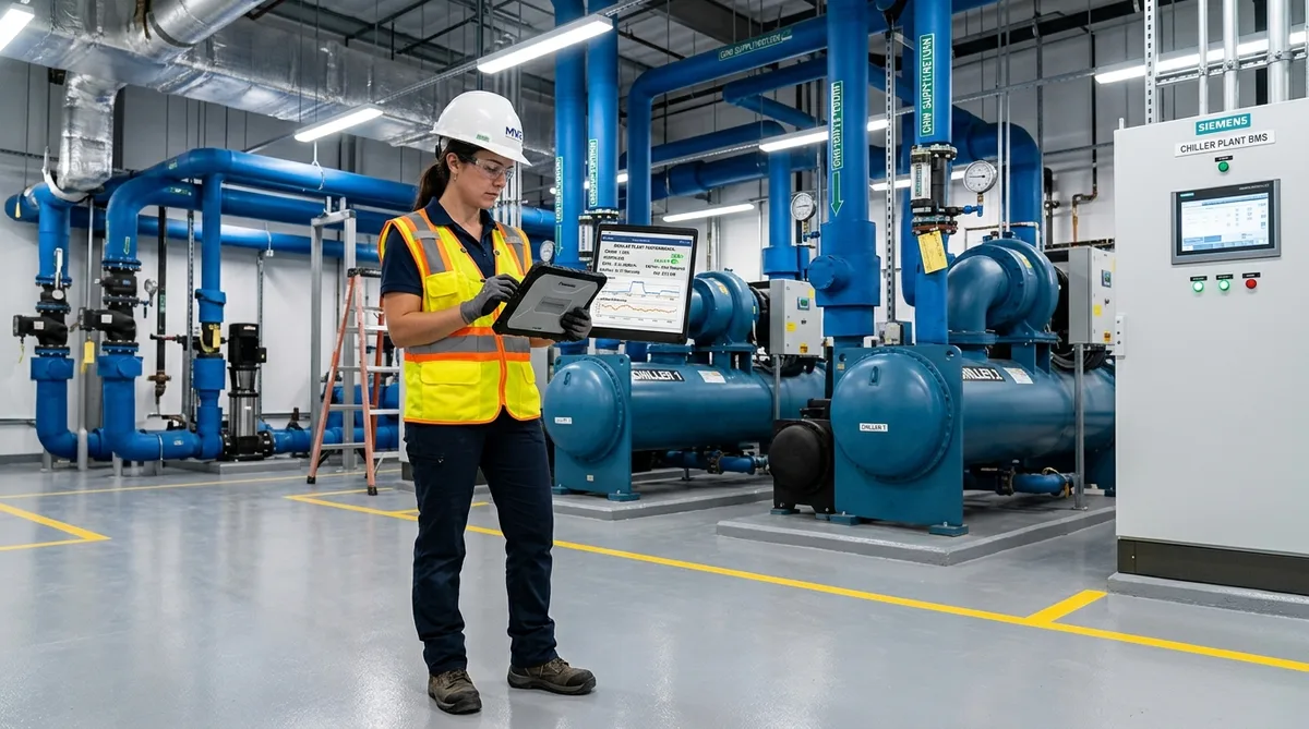 On-site Measurement and Verification (M&V) pairs smart power submetering and thermal flow sensors with calibrated baseline models to prove real-world energy reductions.
The Four Recognized IPMVP M&V Options:
| IPMVP Option | Methodology & Measurement Boundary | Best Retrofit Application | Implementation Cost & Complexity |
|---|---|---|---|
| Option A: Retrofit Isolation (Key Parameter) | Measures key operational parameter (e.g., lighting wattage) while estimating operating hours. | LED lighting upgrades, constant-speed motor replacements. | Low: Simple spot measurements and calculations. |
| Option B: Retrofit Isolation (All Parameters) | Continuously measures all electrical power, flow rates, and temperatures at the component level. | Variable-speed chillers, commercial heat pump water heaters, boiler plants. | Moderate to High: Requires permanent power submeters and BTU flow meters. |
| Option C: Whole-Facility Utility Metering | Evaluates total facility electric and gas utility meters using multivariable regression modeling. | Multi-measure comprehensive retrofits expected to save >10%–15% of whole-building energy. | Low to Moderate: Relies on main utility meters normalized for weather. |
| Option D: Calibrated Simulation | Calibrates whole-building computer models (EnergyPlus/eQUEST) to pre- and post-retrofit utility data. | Deep decarbonization retrofits, major gut rehabilitations, complex interactive envelope/MEP projects. | High: Requires specialized modeling engineers and extensive field data. |
7. Normalization: What Variables Must Be Adjusted in M&V?
To accurately compare post-retrofit utility bills to pre-retrofit baselines, energy engineers apply routine and non-routine mathematical adjustments. Without proper normalization, post-project savings can be masked or falsely exaggerated:
| Normalization Variable | Physical Mechanism | How M&V Normalizes the Data |
|---|---|---|
| Outdoor Temperature (CDD / HDD) | Hotter summers increase chiller kW; colder winters increase boiler fuel. | Weather-regression modeling against Heating Degree Days (HDD) and Cooling Degree Days (CDD). |
| Building Occupancy Density | Higher occupancy increases internal heat, ventilation volume, and domestic hot water. | Per-occupant or per-square-foot baseline adjustments based on badge swipe data. |
| Operating Schedule Extensions | Tenants working late or building operating on weekends increases HVAC runtime. | Schedule-normalized runtime tracking through Building Management Systems (BMS). |
| Tenant Fit-Outs & Server Additions | New IT data closets or commercial kitchens add continuous baseload. | Non-routine baseline adjustments (submetering the new load and subtracting it). |
| Building Floor Area Expansions | Enclosing a terrace or adding conditioned amenity space. | Recalculating baseline Energy Use Intensity (EUI) based on revised gross floor area. |
8. Energy Savings vs. Utility Cost Savings: The Tariff Trap
A critical financial distinction every building executive must recognize is that a model can accurately predict kWh savings while significantly missing cost savings.
In dense urban utility territories like New York City (Con Edison), commercial electricity bills are rarely a simple flat rate per kilowatt-hour. Instead, utility charges are divided into:
- Volumetric Energy Charges ($/kWh): The actual electricity consumed.
- Peak Demand Charges ($/kW): The single highest 15-minute or 30-minute electrical draw during peak billing windows. In NYC, summer demand charges can exceed $30 to $40 per kW!
- Time-of-Use (TOU) Rates: Energy consumed during high-demand summer weekday afternoons costs dramatically more than off-peak overnight power.
If an energy model predicts that a retrofit will reduce energy consumption by 150,000 kWh, but that reduction occurs primarily off-peak (e.g., overnight fan setbacks) while failing to reduce the 2:00 PM peak chiller spike, the building's utility bills will show far less financial savings than projected. Always demand that energy modeling reports separate commodity energy savings (kWh / therms) from tariff-modeled utility cost savings ($).
9. NYC Energy Code Compliance vs. Operational Performance
Under the 2025 NYC Energy Conservation Code (NYCECC), enforced as of March 30, 2026, energy modeling is mandatory when demonstrating compliance through the Total Building Performance Path (Section C407 / ASHRAE 90.1 Appendix G).
The NYC Department of Buildings (DOB) enforces energy modeling to confirm that a proposed building's design meets legal code minimums compared to a standardized baseline. However, the NYC Energy Code explicitly notes that code-compliance approval does not constitute a guarantee of actual utility performance. Code models utilize standardized tenant schedules and fixed internal loads so that all architectural filings are evaluated on an equal regulatory footing.
Connecting Energy Model Accuracy to Local Law 97 Penalties:
Under NYC Local Law 97, covered buildings face annual carbon penalties of $268 per metric ton of CO2e exceeding their assigned emissions caps. When co-op boards and building owners evaluate decarbonization retrofits—such as transitioning from fuel oil to heat pumps—they rely heavily on energy models to prove compliance.
Because actual LL97 penalties are calculated from real post-occupancy utility meters, building owners should run conservative sensitivity analyses. If a retrofit model predicts emissions will drop to 15% below the LL97 cap, but real-world operations deliver only an 80% realization rate, the property could easily slip back into penalty territory. Testing conservative operational scenarios during the design stage protects the building from unexpected compliance fines.
10. What Building Owners Should Demand in an Energy Modeling Deliverable
Never accept an executive summary that simply promises a single percentage savings number. A professional, defensible engineering report must contain:
| Mandatory Report Section | Engineering Deliverables Required | Why Owners Must Review It |
|---|---|---|
| Weather File Specification | Documentation of exact TMY3 or actual weather station data used. | Ensures model reflects local climate rather than generic regional averages. |
| Operating Schedule Narrative | Detailed hour-by-hour schedules for HVAC, lighting, and occupancy. | Verifies that real building hours (including overtime) are modeled. |
| Equipment Part-Load Curves | Manufacturer-specific part-load efficiency curves (e.g., IPLV/NPLV). | Prevents unrealistic assumption of 100% full-load efficiency year-round. |
| ASHRAE 14 Calibration Metrics | Reported NMBE and CV(RMSE) statistical indices against historical bills. | Proves mathematical model validity before forecasting future savings. |
| Sensitivity Scenario Analysis | Three modeled cases: Conservative (10%), Expected (16%), Optimistic (21%). | Enables risk-adjusted financial underwriting and stress testing. |
| Post-Retrofit M&V Plan | Defined IPMVP option, meter locations, and adjustment formulas. | Guarantees a clear mechanism to verify performance after construction. |